Robot Path and Motion Planning
Table of Contents
1. Path Planning 简介
机器人路径规划的基本目标是以最快速度移动到目的地,且不能接触到障碍物。
一般地,机器人路径规划可分为两个层次:一个是 “全局规划” ,它的任务是提前在地图中规划一个从起始位置到达目的位置的线路,例如可以使用 A*算法等;另一个是 “局部规划” ,其主要任务是避免运行过程中遇到的障碍物。如图 1 所示。
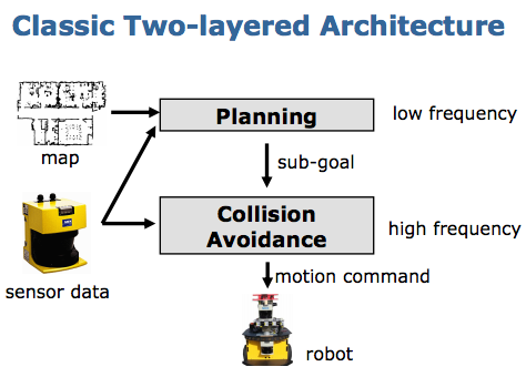
Figure 1: Robot Path Planning Classic Two-layered Architecture
参考:
Planning Algorithms, by Steven M. LaValle: http://planning.cs.uiuc.edu/
http://ais.informatik.uni-freiburg.de/teaching/ss15/robotics/slides/19-pathplanning.pdf
1.1. Path Planning VS. Motion Planning
Path Planning 和 Motion Planning 没有本质区别,有时也混用。不过,一般来说 Path Planning 主要用于无人车、无人机等领域;而 Motion Planning 主要用于机械臂。如,我们想要机器人帮我们抄个菜,这一般归为 Motion Planning 问题。
1.2. Open Motion Planning Library (OMPL)
Open Motion Planning Library (OMPL)是用 C++开发的一个著名的运动规划库。ROS 中的 Moveit!使用了 OMPL。
2. Configuration Space (C-space)
2.1. Configuration, C-space and Workspace
The configuration of a robot system is a complete specification of the position of every point of that system. The configuration space, or C-space, of the robot system is the space of all possible configurations of the system.
The number of degrees of freedom of a robot system is the dimension of the configuration space, or the minimum number of parameters needed to specify the configuration.
We sometimes refer to this ambient space as the workspace.
Usually a configuration is expressed as a vector of positions and orientations.
参考:Principles of Robot Motion - Theory, Algorithms, and Implementations, Chapter 3 - Configuration Space
2.2. Free Space and Obstacle Region
With \(\mathcal{W} = \mathbb{R}^m\) being the workspace, \(\mathcal{O} \in \mathcal{W}\) the set of obstacles, \(\mathcal{A}(q)\) the robot in configuration \(q \in \mathcal{C}\), then
\[\begin{aligned} \mathcal{C}_{free} & := \{ q \in \mathcal{C} \mid \mathcal{A}(q) \cap \mathcal{O} = \emptyset \} \\
\mathcal{C}_{obs} & := C \setminus \mathcal{C}_{free} \\
\end{aligned}\]
常常记 \(q_I\) 为 start configuration,记 \(q_G\) 为 goal configuration,这样 路径规划的目标可以表述为:在 \(\mathcal{C}_{free}\) 中寻找一个从 \(q_I\) 到 \(q_G\) 的路径。
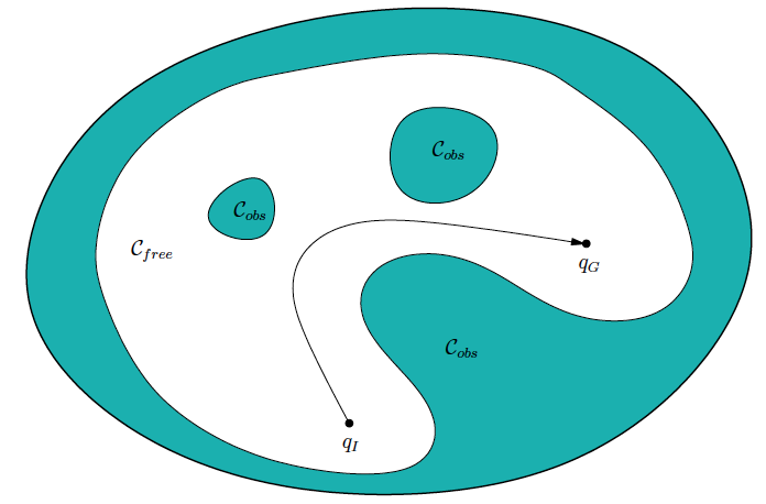
Figure 2: The basic motion planning problem is conceptually very simple using C-space ideas. The task is to find a path from \(q_I\) to \(q_G\) in \(\mathcal{C}_{free}\).
图片摘自:Planning Algorithms, by Steven M. LaValle, 4.3 Configuration Space Obstacles
2.3. Two General Approaches (Sampling-Based Planning and Combinatorial Planning)
求解路径规划问题,有两类方法:
Sampling-Based planning: Avoid the explicit construction of \(\mathcal{C}_{obs}\), uses collision-detection to probe and incrementally search the C-space for solution.
Combinatorial planning: Characterizes \(\mathcal{C}_{free}\) explicitely by capturing the connectivity of \(\mathcal{C}_{free}\) into a graph and finds solutions using search. Combinatorial planning find paths through the continuous configuration space without resorting to approximations. Combinatorial planning algorithms are alternatively referred to as exact algorithms.
参考:
Planning Algorithms, by Steven M. LaValle, Chapter 5 Sampling-Based Motion Planning
Planning Algorithms, by Steven M. LaValle, Chapter 6 Combinatorial Motion Planning
3. Sampling-Based Motion Planning
参考:Planning Algorithms, by Steven M. LaValle, 5. Sampling-Based Motion Planning
3.1. Rapidly-exploring Random Tree (RRT)
3.2. Probabilistic road map (PRM)
4. Collision Avoidance
机器人避障是路径规划的重要组成部分,相关算法有很多,如:
- Bug algorithm
- Vector field histogram
- The bubble band technique
- Curvature velocity techniques
- Dynamic window approaches
- The Schlegel approach to obstacle avoidance
- The ASL approach
- Nearness diagram
- Gradient method
- Adding dynamic constraints
参考:Introduction to Autonomous Mobile Robots, by Roland Siegwart, Illah Reza Nourbakhsh, 6.2.2 Obstacle avoidance
4.1. Bug Algorithm
The Bug algorithm is perhaps the simplest obstacle avoidance algorithm one could imagine. The basic idea is to follow the contour of each obstacle in the robot’s way and thus circumnavigate it.
With Bug1, the robot fully circles the object first, then departs from the point with the shortest distance toward the goal. This approach is, of course, very inefficient but guarantees that the robot will reach any reachable goal.
With Bug2 the robot begins to follow the object’s contour, but departs immediately when it is able to move directly toward the goal. In general this improved Bug algorithm will have significantly shorter total robot travel.
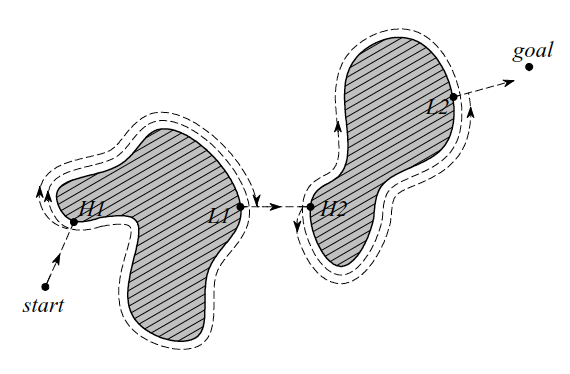
Figure 3: Bug1 algorithm with H1, H2, hit points, and L1, L2, leave points
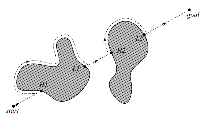
Figure 4: Bug2 algorithm with H1, H2, hit points, and L1, L2, leave points
4.2. Dynamic Window Approache
In robotics motion planning, the dynamic window approach is a real-time collision avoidance strategy for mobile robots developed by Dieter Fox, Wolfram Burgard, and Sebastian Thrun in 1997.
动态窗口法的主要思想是 在速度空间 \((v, \omega)\) 中采样多组速度,模拟机器人在这些速度下一定时间内的轨迹。对这些轨迹进行评价,选取最优的轨迹所对应的速度来驱动机器人运动。 名字“动态窗口”的含义是依据机器人的加减速性能限定速度的采样空间在一个可行的动态范围内。
参考:
作者原始论文:https://www.ri.cmu.edu/pub_files/pub1/fox_dieter_1997_1/fox_dieter_1997_1.pdf
机器人局部避障的动态窗口法(dynamic window approach): http://blog.csdn.net/heyijia0327/article/details/44983551
4.2.1. 动态窗口法的速度采样空间
下面介绍如何确定速度 \((v, \omega)\) 的采样空间。
(1) 为了在最大的减速度条件下,确保机器人能够在碰到障碍物之前停下来,其速度不能太快,必须有个限制。假设 \(V_a\) 表示不会碰到障碍物的所有速度的集合,则:
\[V_a = \left\{ (v, \omega) \mid v \le \sqrt{2 \cdot \text{dist}(v, \omega) \cdot a_{trans}} \wedge \omega \le \sqrt{2 \cdot \text{dist}(v, \omega) \cdot a_{rot}} \right\}\]
上式中,\(a_{trans}\) 是最大的加速度, \(a_{rot}\) 是最大的角加速度。 \(\text{dist}(v, \omega)\) 是速度 \((v, \omega)\) 对应轨迹上机器人与最近的障碍物之间的距离,如图 5 所示的弧线所示。
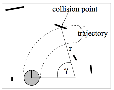
Figure 5: Determination of the distance
说明:上面结论容易由物理公式 \(S = v_0 t + \frac{1}{2}a t^2 = \frac{v_t^2 - v_0^2}{2a}\) 推导而来(令 \(v_t = 0\) ,可得 \(v_0 = \sqrt{- 2 a S}\) ,相差正负符号说明这里是减速度)。
(2) 由于电机性能限制,存在一个 动态窗口,在该窗口内的速度是机器人能实际达到的速度。 假设 \(V_d\) 表示这个动态窗口(当前机器人在 \(\Delta t\) 内可以达到的速度的集合),则:
\[V_d = \left\{ (v, \omega) \mid v \in [v_c - a_{trans} \cdot \Delta t, v_c + a_{trans} \cdot \Delta t] \wedge \omega \in [\omega_c - a_{rot} \cdot \Delta t , \omega_c + a_{rot} \cdot \Delta t ] \right\}\]
上式中, \((v_c, \omega_c)\) 是机器人当前的速度。
(3) 机器人自身有一个速度限制,设为 \(V_s\) 。
最后,机器人速度的采样空间可以这样表述:
\[V_r = V_s \cap V_a \cap V_d\]
其中,
\(V_s\) = all possible speeds of the robot.
\(V_a\) = obstacle free area.
\(V_d\) = speeds reachable within a certain time frame based on possible accelerations.
Figure 6: 速度采样空间
4.2.2. 动态窗口法的评价函数
在速度空间 \(V_r\) 中采样得到了很多可行的速度后,如何选择一条最合适的呢?
每一个采样速度都会有一个对应的预计轨迹。采用评价函数的方式给每个轨迹打分,分数最高的轨迹对应的速度就是我们的选择。原始论文中采用的评价函数为:
\[G(v, \omega) = \sigma \left(\alpha \cdot \text{heading}(v, \omega) + \beta \cdot \text{dist}(v, \omega) + \gamma \cdot \text{velocity}(v, \omega) \right)\]
其中,
(1) \(\text{heading}(v, \omega)\) 用来评价在当前采样速度下,机器人达到预计轨迹末端时朝向和目标朝向之间的角度的差距。 \(\text{heading}(v, \omega)\) 满足角度差距越小分数越高即可。
(2) \(\text{dist}(v, \omega)\) 用来评价在当前采样速度下,机器人预计轨迹和最近的障碍物之间的距离。
(3) \(\text{velocity}(v, \omega)\) 用来标记采样速度(我们希望速度越快越好,可尽快到达目标)。
4.2.3. 动态窗口法的不足
使用动态窗口法的机器人有一个不足之处:Robot does not slow down early enough to enter the doorway.
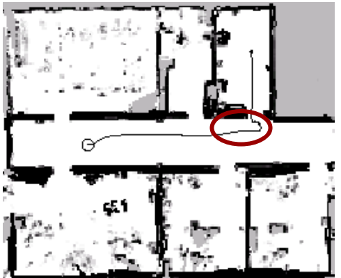
Figure 7: Problems of Dynamic Window Approache
参考:http://ais.informatik.uni-freiburg.de/teaching/ss15/robotics/slides/19-pathplanning.pdf