Spark

1. Spark 简介
2. 弹性分布式数据集（RDD）
3. 共享变量
- 3.1. 广播变量（只读）
- 3.2. 累加器
4. 参考

1. Spark 简介

Spark 是一个开源框架，作为计算引擎，它把程序分发到集群中的许多机器，同时提供了一个优雅的编程模型。 Spark 源自加州大学伯克利分校的 AMPLab，现在已被捐献给了 Apache 软件基金会。可以这么说，对于数据科学家而言，真正让分布式编程进入寻常百姓家的开源软件， Spark 是第一个。

了解 Spark 的最好办法莫过于了解相比于它的前辈（即 Apache Hadoop 的 MapReduce），Spark 有哪些进步。 MapReduce 革新了海量数据的计算方式，为运行在成百上千台机器上的并行程序提供了简单的编程模型。MapReduce 引擎几乎可以做到线性扩展：随着数据量的增加，可以通过增加多的计算机来保持作业时间不变。而且 MapReduce 是健壮的。故障虽然在单台机器上很少出现，但在数千个节点的集群上却总是出现。对于这种情况，MapReduce 也能妥善处理。它将工作拆分成多个小任务，能优雅地处理失败的任务，并且不影响任务所属作业的正确执行。

Spark 继承了 MapReduce 的线性扩展性和容错性，同时对它做了一些重量级扩展。首先，Spark 摒弃了 MapReduce 先 map 再 reduce 这样的严格方式，Spark 引擎可以执行更通用的有向无环图（directed acyclic graph，DAG）算子。这就意味着，在 MapReduce 中需要将中间结果写入分布式文件系统时，Spark 能将中间结果直接传到流水作业线的下一步。

再次，Spark 扩展了前辈们的内存计算能力。 它能将作业与作业之间产生的大规模的工作数据集存储在内存中。这样后续步骤如果需要相同数据集就不必重新计算或从磁盘加载。这个特性使 Spark 可以应用于以前分布式处理引擎无法胜任的应用场景中。Spark 非常适用于涉及大量迭代的算法，这些算法需要多次遍历相同的数据集。Spark 也适用于反应式（reactive）应用，这些应用需要扫描大量内存数据并快速响应用户的查询。

1.1. 安装

从下载页面（https://spark.apache.org/downloads.html ）下载一个稳定版本的 Spark 二进制发行包（应当选择与正在使用的 Hadoop 发行版匹配的版本），然后在合适的位置解压缩该文件包：

$ tar xzf spark-2.4.5-bin-hadoop2.7.tgz

为了方便起见，可以把 Spark 的二进制文件路径添加到你的路径中，如下所示：

$ export SPARK_HOME=~/spark-2.4.5-bin-hadoop2.7
$ export PATH=$PATH:$SPARK_HOME/bin

执行 spark-shell 可以启动添加了 Spark 功能的 Scala REPL 交互式解释器。如：

$ spark-shell
Using Spark's default log4j profile: org/apache/spark/log4j-defaults.properties
Setting default log level to "WARN".
To adjust logging level use sc.setLogLevel(newLevel). For SparkR, use setLogLevel(newLevel).
Spark context Web UI available at http://192.168.1.4:4040
Spark context available as 'sc' (master = local[*], app id = local-1585241995961).
Spark session available as 'spark'.
Welcome to
      ____              __
     / __/__  ___ _____/ /__
    _\ \/ _ \/ _ `/ __/  '_/
   /___/ .__/\_,_/_/ /_/\_\   version 2.4.5
      /_/

Using Scala version 2.11.12 (Java HotSpot(TM) 64-Bit Server VM, Java 1.8.0_66)
Type in expressions to have them evaluated.
Type :help for more information.

scala>

执行 pyspark 可以启动 Spark Python Shell。

1.2. 集群部署模式

Spark 支持下面几种集群部署模式：
1、Standalone Mode
2、Apache Mesos
3、Hadoop YARN
4、Kubernetes

其中，独立模式自带完整的服务，方便测试使用。

1.3. 第一个应用

下面以统计文本文件（如“spark-2.4.5-bin-hadoop2.7/README.md”）中分别包含字母“a”和“b”的“行数”为例介绍一下 Spark 的使用。

参考：https://spark.apache.org/docs/latest/quick-start.html

1.3.1. 交互环境

在 spark-shell 交互环境下，完成上面任务比较容易：

scala> val lines = spark.read.textFile("/path/to/spark-2.4.5-bin-hadoop2.7/README.md")
lines: org.apache.spark.sql.Dataset[String] = [value: string]

scala> lines.filter(line => line.contains("a")).count()
res4: Long = 61

scala> lines.filter(line => line.contains("b")).count()
res5: Long = 30

1.3.2. 编写 Self-Contained 应用

下面介绍使用“Self-Contained 应用”完成前面的任务。

准备 scala 源码（SimpleApp.scala），内容如下：

/* SimpleApp.scala */
import org.apache.spark.sql.SparkSession

object SimpleApp {
  def main(args: Array[String]) {
    val logFile = "/path/to/spark-2.4.5-bin-hadoop2.7/README.md"    // Should be some file on your system
    val spark = SparkSession.builder.appName("Simple Application").getOrCreate()
    val lines = spark.read.textFile(logFile).cache()   // 使用cache把文本内容缓存到内存中
    val numAs = lines.filter(line => line.contains("a")).count()
    val numBs = lines.filter(line => line.contains("b")).count()
    println(s"Lines with a: $numAs, Lines with b: $numBs")
    spark.stop()
  }
}

准备 sbt 配置文件（build.sbt），把 Spark 相关依赖库加入到其 libraryDependencies 中，内容如下：

name := "Simple Project"

version := "1.0"

// 下载版本要和 spark 使用的 scala 版本精确对应
scalaVersion := "2.11.12"

libraryDependencies += "org.apache.spark" %% "spark-sql" % "2.4.5"

源码的目录结构如下：

# Your directory layout should look like this
$ find .
.
./build.sbt
./src
./src/main
./src/main/scala
./src/main/scala/SimpleApp.scala

# Package a jar containing your application
$ sbt package
...
[info] Packaging {..}/{..}/target/scala-2.11/simple-project_2.11-1.0.jar

使用 sbt package 编译打包成功后，会生成“target/scala-2.11/simple-project_2.11-1.0.jar”。

使用 spark-submit 提交到 Spark 中执行，可以看到下面结果：

$ spark-submit \
  --class "SimpleApp" \
  --master "local[4]" \
  target/scala-2.11/simple-project_2.11-1.0.jar
......
Lines with a: 61, Lines with b: 30
......

1.4. SparkContext, SparkSession

SparkContext 是调用 Spark 功能的一个主要入口。 一个 SparkContext 对象代表与一个 Spark 集群的连接。

SparkSession 在 Spark 2.X 中引入，现在是 Spark 的新入口点，使开发人员可以简化对不同上下文的访问。如果正在使用 Spark 2.0 或更高版本，建议使用 SparkSession。

下面是创建 SparkSession 的例子：

//Creating a SparkSession in Scala
import org.apache.spark.sql.SparkSession

val spark = SparkSession.builder().appName("Databricks Spark Example")
     .config("spark.sql.warehouse.dir", "/user/hive/warehouse")
     .getOrCreate()

执行 spark-shell 打开 Scala 交互环境时，默认提供了名为“sc”的预配置 SparkContext，和名为“spark”的预配置 SparkSession，你可以在启动时看到下面提示：

$ spark-shell
......
Spark context available as 'sc' (master = local[*], app id = local-1585241995961).
Spark session available as 'spark'.
......
scala>

2. 弹性分布式数据集（RDD）

弹性分布式数据集（RDD，Resilient Distributed Dataset）是对数据集的抽象封装，开发人员可以通过 RDD 提供的开发接口来访问和操纵数据集合，而无须了解数据的存储介质（内存或磁盘）、文件系统（本地文件系统、HDFS 或 Tachyon）、存储节点（本地或远程节点）等诸多实现细节。Spark 中的 RDD 具有容错性，即当某个节点或任务失败时（由用户代码错误之外的原因引起，如硬件故障、网络不通等），RDD 会在余下的节点上自动重建，以便最终完成任务。

Spark 的整个计算过程都是围绕 RDD 来进行。

参考：RDD Programming Guide

2.1. 创建 RDD

可以从现有的集合中创建 RDD，如：

val collection = List("a", "b", "c", "d", "e")      // 创建集合
val rddFromCollection = sc.parallelize(collection)  // 由集合创建 RDD

也可以从本地或 HDFS 中创建 RDD，如：

val rddFromTextFile = sc.textFile("LICENSE")                   // 从本地文件创建 RDD
val rddFromTextFileHDFS = sc.textFile("hdfs://input/LICENSE ") // 从 HDFS 文件创建 RDD

RDD 是只读的，内部的数据无法被修改 ，可以通过数据转换（后面会介绍）得到新的 RDD，这不会影响原来的 RDD 内容。

2.2. 操作 RDD（Transformation 和 Action）

创建 RDD 后，可以对 RDD 进行操作。操作可以分为两类：Transformation 和 Action。如图 1 （摘自：http://www.ijceronline.com/papers/Vol8_issue7/Version-1/C0807011019.pdf）所示。

Figure 1: RDD Operations

Transformation 返回值还是一个 RDD。 然后这个 RDD 又可以进行另外一次转换（Transformation），这个过程是分布式的。Action 返回值不是一个 RDD，它要么是一个 Scala 的普通集合，要么是一个值，要么是空。 Action 的返回值返回给 Driver 程序（启动 SparkContext 的程序）或者存储到文件。

Transaction 是“惰性执行”（或者称为“延迟计算”）的，惰性执行表示真正需要时才被执行，这里是在需要具体的 Action 去触发才会开始执行，每个 Action 的触发都会提交一个 Job。

Job 和 Stage 的关系是： 一个 Action 触发一个 Job。一个 Job 会被拆为多组任务，每组任务称为一个 Stage。

2.2.1. Transformation

表 1 总结了 RDD 的一些常用 Transformation。

Table 1: RDD Transformation
Transformation	Meaning
map(func)	Return a new distributed dataset formed by passing each element of the source through a function func.
filter(func)	Return a new dataset formed by selecting those elements of the source on which func returns true.
flatMap(func)	Similar to map, but each input item can be mapped to 0 or more output items (so func should return a Seq rather than a single item).
mapPartitions(func)	Similar to map, but runs separately on each partition (block) of the RDD, so func must be of type Iterator<T> => Iterator<U> when running on an RDD of type T.
mapPartitionsWithIndex(func)	Similar to mapPartitions, but also provides func with an integer value representing the index of the partition, so func must be of type (Int, Iterator<T>) => Iterator<U> when running on an RDD of type T.
sample(withReplacement, fraction, seed)	Sample a fraction fraction of the data, with or without replacement, using a given random number generator seed.
union(otherDataset)	Return a new dataset that contains the union of the elements in the source dataset and the argument.
intersection(otherDataset)	Return a new RDD that contains the intersection of elements in the source dataset and the argument.
distinct([numPartitions]))	Return a new dataset that contains the distinct elements of the source dataset.
groupByKey([numPartitions])	When called on a dataset of (K, V) pairs, returns a dataset of (K, Iterable<V>) pairs. Note: If you are grouping in order to perform an aggregation (such as a sum or average) over each key, using reduceByKey or aggregateByKey will yield much better performance. Note: By default, the level of parallelism in the output depends on the number of partitions of the parent RDD. You can pass an optional numPartitions argument to set a different number of tasks.
reduceByKey(func, [numPartitions])	When called on a dataset of (K, V) pairs, returns a dataset of (K, V) pairs where the values for each key are aggregated using the given reduce function func, which must be of type (V,V) => V. Like in groupByKey, the number of reduce tasks is configurable through an optional second argument.
aggregateByKey(zeroValue)(seqOp, combOp, [numPartitions])	When called on a dataset of (K, V) pairs, returns a dataset of (K, U) pairs where the values for each key are aggregated using the given combine functions and a neutral "zero" value. Allows an aggregated value type that is different than the input value type, while avoiding unnecessary allocations. Like in groupByKey, the number of reduce tasks is configurable through an optional second argument.
sortByKey([ascending], [numPartitions])	When called on a dataset of (K, V) pairs where K implements Ordered, returns a dataset of (K, V) pairs sorted by keys in ascending or descending order, as specified in the boolean ascending argument.
join(otherDataset, [numPartitions])	When called on datasets of type (K, V) and (K, W), returns a dataset of (K, (V, W)) pairs with all pairs of elements for each key. Outer joins are supported through leftOuterJoin, rightOuterJoin, and fullOuterJoin.
cogroup(otherDataset, [numPartitions])	When called on datasets of type (K, V) and (K, W), returns a dataset of (K, (Iterable<V>, Iterable<W>)) tuples. This operation is also called groupWith.
cartesian(otherDataset)	When called on datasets of types T and U, returns a dataset of (T, U) pairs (all pairs of elements).
pipe(command, [envVars])	Pipe each partition of the RDD through a shell command, e.g. a Perl or bash script. RDD elements are written to the process's stdin and lines output to its stdout are returned as an RDD of strings.
coalesce(numPartitions)	Decrease the number of partitions in the RDD to numPartitions. Useful for running operations more efficiently after filtering down a large dataset.
repartition(numPartitions)	Reshuffle the data in the RDD randomly to create either more or fewer partitions and balance it across them. This always shuffles all data over the network.
repartitionAndSortWithinPartitions(partitioner)	Repartition the RDD according to the given partitioner and, within each resulting partition, sort records by their keys. This is more efficient than calling repartition and then sorting within each partition because it can push the sorting down into the shuffle machinery.

2.2.2. Action

表 2 总结了 RDD 的一些常用 Action。

Table 2: RDD Action
Action	Meaning
reduce(func)	Aggregate the elements of the dataset using a function func (which takes two arguments and returns one). The function should be commutative and associative so that it can be computed correctly in parallel.
collect()	Return all the elements of the dataset as an array at the driver program. This is usually useful after a filter or other operation that returns a sufficiently small subset of the data.
count()	Return the number of elements in the dataset.
first()	Return the first element of the dataset (similar to take(1)).
take(n)	Return an array with the first n elements of the dataset.
takeSample(withReplacement, num, [seed])	Return an array with a random sample of num elements of the dataset, with or without replacement, optionally pre-specifying a random number generator seed.
takeOrdered(n, [ordering])	Return the first n elements of the RDD using either their natural order or a custom comparator.
saveAsTextFile(path)	Write the elements of the dataset as a text file (or set of text files) in a given directory in the local filesystem, HDFS or any other Hadoop-supported file system. Spark will call toString on each element to convert it to a line of text in the file.
saveAsSequenceFile(path) (Java and Scala)	Write the elements of the dataset as a Hadoop SequenceFile in a given path in the local filesystem, HDFS or any other Hadoop-supported file system. This is available on RDDs of key-value pairs that implement Hadoop's Writable interface. In Scala, it is also available on types that are implicitly convertible to Writable (Spark includes conversions for basic types like Int, Double, String, etc).
saveAsObjectFile(path) (Java and Scala)	Write the elements of the dataset in a simple format using Java serialization, which can then be loaded using SparkContext.objectFile().
countByKey()	Only available on RDDs of type (K, V). Returns a hashmap of (K, Int) pairs with the count of each key.
foreach(func)	Run a function func on each element of the dataset. This is usually done for side effects such as updating an Accumulator or interacting with external storage systems. Note: modifying variables other than Accumulators outside of the foreach() may result in undefined behavior. See Understanding closures for more details.

2.3. RDD 分区

在 RDD 内部，如何表示并行计算的一个计算单元呢？答案是使用分区（Partition）。 RDD 内部的数据集合在逻辑上（在物理上则不一定）被划分成多个分片，这样的每一个分片称为分区，分区的个数会决定并行计算的粒度，而每一个分区数值的计算都是在一个单独的任务中进行，因此任务的个数，也是由 RDD（准确来说是最后一个作业的最后一个 RDD）分区的个数决定的。

创建 RDD 时可以手动指定分区的个数，例如 sc.parallelize(Array(1, 2, 3, 4, 5), 2) 表示创建得到的 RDD 分区个数为 2，在没有指定分区个数的情况下，Spark 会根据集群部署模式，来确定一个分区个数默认值。

在 RDD 转换操作中，转换后得到的 RDD 的分区个数会根据“转换操作中对应的多个 RDD 之间的依赖关系确定”。

2.3.1. RDD 的窄依赖和宽依赖

在一次转换操作中，创建得到的新 RDD 称为“子 RDD”，提供数据的 RDD 称为“父 RDD”，父 RDD 可能会存在多个。 子 RDD 与父 RDD之间的关系称为依赖关系。

Spark 将依赖关系进一步分为两类，分别是窄依赖（Narrow Dependency）和宽依赖（Wide Dependency）。 宽依赖又称为 Shuffle 依赖（Shuffle Dependency）。

2.3.1.1. 窄依赖

窄依赖指父 RDD 的每个分区只被子 RDD 的一个分区所使用，子 RDD 分区通常对应常数个父 RDD 分区。换句话说， 窄依赖中，父 RDD 中，一个分区内的数据是不能被分割的，必须整个交付给子 RDD 中的一个分区。 如图 2 所示。

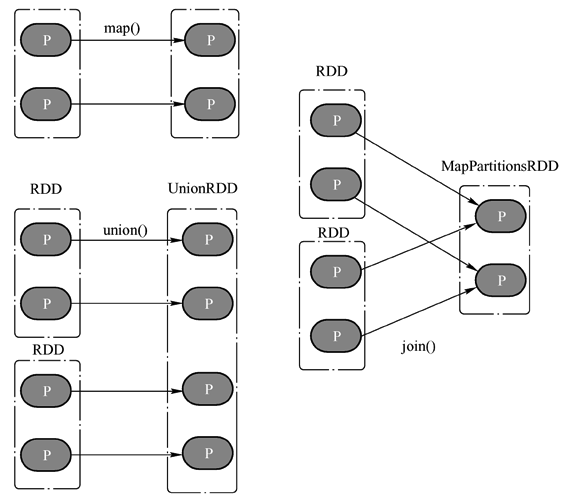
Figure 2: 窄依赖（父 RDD 分区内的数据没有被分割）

2.3.1.2. 宽依赖（Shuffle）

宽依赖中，父 RDD 中的分区可能会被多个子 RDD 分区使用。父 RDD 中一个分区内的数据会被分割，发送给子 RDD 的所有分区。如图 3 所示。

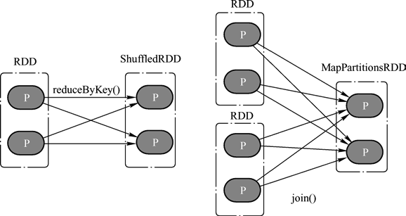
Figure 3: 宽依赖（父 RDD 分区内的数据被发送给子 RDD 的多个分区）

依赖关系是两个 RDD 之间的依赖，因此若一次转换操作中父 RDD 有多个，则可能会“同时包含窄依赖和宽依赖”，如图 4 所示的 join 操作，RDD a 和 RDD c 采用了相同的分区器，两个 RDD 之间是窄依赖，Rdd b 的分区器与 RDD c 有所不同，因此它们之间是宽依赖。

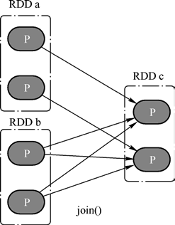
Figure 4: 同时包含窄依赖和宽依赖（a 和 c 采用了相同的分区器，b 和 c 采用的分区器不同）

2.3.2. 分区器

分区器能够间接决定 RDD 中分区的数量和分区内部数据记录的个数，因此选择合适的分区器能够有效提高并行计算的性能。Spark 内置了两类分区器，分别是哈希分区器（Hash Partitioner）和范围分区器（Range Partitioner），此外，开发者还可以根据实际需求编写自己的分区器。

2.3.2.1. 哈希分区器

哈希分区器用下面方法来确定其分配到子 RDD 中的哪一个分区：取键值的 hashCode，除上子 RDD 分区个数，取余即可。如 5 所示。

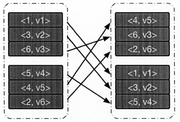
Figure 5: 哈希分区器例子

2.3.2.2. 范围分区器

哈希分析器有个缺点：它不关心键值的分布情况，其散列到不同分区的概率会因数据而异，个别情况下会导致一部分分区分配到的数据多，一部分则比较少。范围分区器则在一定程度上避免这个问题， 范围分区器争取将所有的分区尽可能分配得到“相同多的数据”，并且所有分区内数据的“上界是有序的”。

图 6 是使用范围分区器进行分区的一个示例。

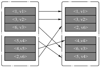
Figure 6: 范围分区器例子

范围分区器的原理与 Apache Hadoop 上的 TeraSort 算法有些类似，范围分区器希望能够将所有键值划分成几个数据块（数目等于子 RDD 的分区个数），找出每个数据块的边界，每个数据块边界范围内，数据的个数应该是基本相等的，根据边界可以将键值对记录指派给特定的分区。

2.3.2.3. 默认分区器

若开发者没有明确指明使用的分区器，则 Spark 会使用默认分区器：Spark 会把父 RDD 和子 RDD 按照 RDD 的分区个数从大到小进行排序，只要其中有一个 RDD 指定了分区器，则子 RDD 的分区器将与其一致，若所有的 RDD 都没有指定分区器，则采用“哈希分区器”，分区个数等于 spark.default.parallelism 。

2.4. RDD 持久化

在 Spark 计算过程中，中间数据默认不会被保存，每次的动作（Action）操作都会对数据重复计算 ，某些计算量比较大的操作可能会影响到系统的运算效率，因此 Spark 允许在转换过程中手动将某些会被频繁使用的RDD 执行持久化操作，持久化后的数据可以被存储在内存、磁盘或者 Tachyon 当中，这将使得后续的动作（Actions）变得更加迅速（通常快 10 倍以上）。

通过调用 RDD 提供的 cache 或 persist 函数即可实现数据的持久化，persist 函数需要指定存储级别（Storage Level），cache 等价于采用 MEMORY_ONLY 存储级别的 persist 函数。Spark 提供的存储级别及其含义如表 3 所示。

Table 3: Spark 存储级别
存储级别	含义
MEMORY_ONLY	把 RDD 以非序列化状态存储在内存中，如果内存空间不够，则有些分区数据会在需要的时候进行计算得到
MEMORY_AND_DISK	把 RDD 以非序列化存储在内存中，如果内存空间不够，则存储在硬盘中
MEMORY_ONLY_SER	把 RDD 以 Java 对象序列化储存在内存中，序列化后占用空间更小
MEMORY_AND_DISK_SER	类似 MEMORY_ONLY_SER，区别是当内存不够的时候会把 RDD 持久化到磁盘中，而不是在需要它们的时候实时计算
DISK_ONLY	只把 RDD 存储到磁盘中
MEMORY_ONLY_2	类似 MEMORY_ONLY，不同的是会复制一个副本到另一个集群节点
MEMORY_AND_DISK_2	类似 MEMORY_AND_DISK，不同的是会复制一个副本到另一个集群节点

2.5. RDD 检查点

DAG 中 Lineage 如果太长，重计算的时候开销会很大，故使用检查点机制，将计算过程持久化到磁盘，这样如果出现计算故障就可以在检查点开始重计算，而不需要从头开始。RDD 的检查点（checkpoint）机制类似持久化机制中的 persist(StorageLevel.DISK_ONLY) ，数据会被存储在磁盘当中，两者最大的区别在于： 持久化机制所存储的数据，在驱动程序运行结束之后会被自动清除；检查点机制则会将数据永久存储在磁盘当中，如果不手动删除，数据会一直存在。 换句话说，检查点机制存储的数据能够被下一次运行的应用程序所使用。

检查点的使用与持久化类似，调用 RDD 的 checkpoint 方法即可。

参考：https://spark.apache.org/docs/latest/streaming-programming-guide.html#checkpointing

3. 共享变量

通常情况下，一个应用程序在运行的时候会被划分成分布在不同执行节点之上的多个任务，从而提高运算的速度，每个任务都会有一份独立的程序变量拷贝，彼此之间互不干扰，然而在某些情况下任务之间需要相互共享变量，Apache Spark 提供了两类“共享变量”（Shared Variables），它们分别是广播变量（Broadcast Variable）和累加器（Accumulators）。

3.1. 广播变量（只读）

广播变量（Broadcast Variables）允许用户将一个只读变量缓存到每一台机器之上，而不像传统变量一样，复制到每一个任务当中，同一台机器上的不同任务可以共享该变量值。

对于变量 v ，只需要调用 SparkContext.broadcast(v) 即可得到变量 v 的广播变量（假设记为 broadcastVar ），而通过调用 broadcastVar 的 value 方法即可取得变量值。下面是代码示例：

scala> val broadcastVar = sc.broadcast(Array(1, 2, 3))
broadcastVar: org.apache.spark.broadcast.Broadcast[Array[Int]] = Broadcast(0)

scala> broadcastVar.value
res0: Array[Int] = Array(1, 2, 3)

3.2. 累加器

累加器（Accumulators）是另外一种共享变量。累加器变量只能执行加法操作，但其支持并行操作，这意味着不同任务多次对累加器执行加法操作后，加法器最后的值（也是通过其 value 方法得到）等于所有累加的和。累加器的值只能被 Driver 程序访问，集群中的任务无法访问该值。如：

scala> val accum = sc.longAccumulator("My Accumulator")
accum: org.apache.spark.util.LongAccumulator = LongAccumulator(id: 0, name: Some(My Accumulator), value: 0)

scala> sc.parallelize(Array(1, 2, 3, 4)).foreach(x => accum.add(x))
...
10/09/29 18:41:08 INFO SparkContext: Tasks finished in 0.317106 s

scala> accum.value
res2: Long = 10

累加器与广播变量的关键不同是后者只能读取而前者却可累加。

4. 参考

《Spark原理、机制及应用》
《Spark高级数据分析（第2版）》