Graphviz

1. Graphviz 简介
- 1.1. DOT Language
- 1.2. dot 命令
2. Graphviz 实例
3. Tips
- 3.1. 设置连接点的位置
- 3.2. 圆角矩形（shape=Mrecord）

1. Graphviz 简介

Graphviz 是一款由 AT&T 实验室开源的可视化图形工具，可以很方便的用来绘制结构化的图形网络，支持多种格式输出。

Graphviz 的画图实例可参考：https://graphviz.org/gallery/

1.1. DOT Language

Graphviz 采用脚本语言 DOT 来定义输入。DOT 的语法如下：

     graph : [ strict ] (graph | digraph) [ ID ] '{' stmt_list '}'
 stmt_list : [ stmt [ ';' ] stmt_list ]
      stmt : node_stmt
           | edge_stmt
           | attr_stmt
           | ID '=' ID
           | subgraph
 attr_stmt : (graph | node | edge) attr_list
 attr_list : '[' [ a_list ] ']' [ attr_list ]
    a_list : ID '=' ID [ (';' | ',') ] [ a_list ]
 edge_stmt : (node_id | subgraph) edgeRHS [ attr_list ]
   edgeRHS : edgeop (node_id | subgraph) [ edgeRHS ]
 node_stmt : node_id [ attr_list ]
   node_id : ID [ port ]
      port : ':' ID [ ':' compass_pt ]
           | ':' compass_pt
  subgraph : [ subgraph [ ID ] ] '{' stmt_list '}'
compass_pt : (n | ne | e | se | s | sw | w | nw | c | _)

The keywords node, edge, graph, digraph, subgraph, and strict are case-independent. Note also that the allowed compass point values are not keywords, so these strings can be used elsewhere as ordinary identifiers and, conversely, the parser will actually accept any identifier.

参考：http://www.graphviz.org/content/dot-language

1.2. dot 命令

dot 一般用于绘制有向图，无向图则可用 neato 或者 fdp，可以互相通用，差别在于 dot 生成的有向图效果要好点，neato 和 fdp 生成的无向图效果要好点。其他的如辐射状的图形可用 twopi，圆形的可用 circo。它们的命令行参数都是一致的，只是所用的算法不一而已。

实例：无向图（graph）

$ cat example1.dot
graph example1 {
Server1 -- Server2
Server1 -- Server3
Server2 -- Server4
Server2 -- Server5
}
$ dot -Tpng  example1.dot  -o dot_example1.png

生成的图片 dot_example1.png 如图 1 所示。

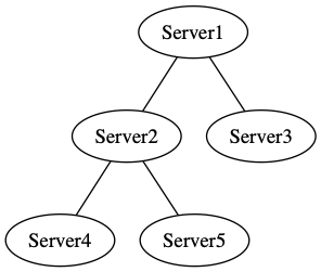
Figure 1: dot 绘制无向图

实例：有向图（digraph）

$ cat example2.dot
digraph example2 {
Server1 -> Server2
Server1 -> Server3
Server2 -> Server4
Server2 -> Server5
}
$ dot -Tpng  example2.dot  -o dot_example2.png

生成的图片 dot_example2.png 如图 2 所示。

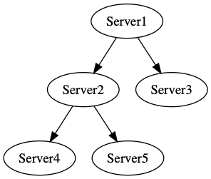
Figure 2: dot 绘制有向图

2. Graphviz 实例

下面介绍一些 graphviz 的实例，主要摘自：Drawing graphs with dot。

2.1. 节点和边的属性

默认地，所有节点用属性 shape=ellipse, width=.75, height=.5 进行绘制。

考虑 dot 文件：

digraph G {
  main -> init;
  main -> parse;
  main -> cleanup;
  parse -> execute;
  execute -> make_string;
  execute -> printf
  init -> make_string;
  main -> printf;
  execute -> compare;
}

上面代码可以生成图 3。

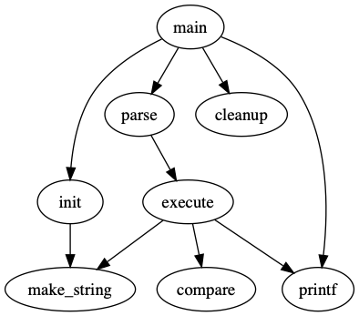
Figure 3: Example

通过下面指令可以设置“边”和“节点”的默认属性：

edge [key1=val1];  // 设置从该指令后，边的属性 key1 为 val1
node [key1=val1];  // 设置从该指令后，节点的属性 key1 为 val1

如下面 dot 代码中的第 6、7 行就是设置“边”和“节点”的默认属性；也可以单独修改某边的属性（第 11 行），或者某节点的属性（第 13 行）：

 1: digraph G {
 2:   main -> init;
 3:   main -> parse;
 4:   main -> cleanup;
 5:   parse -> execute;
 6:   edge [color=red];                                   // 从后面开始，设置边的默认属性
 7:   node [shape=box, style=filled, color=".7 .3 1.0"];  // 从后面开始，设置节点的默认属性
 8:   execute -> make_string;
 9:   execute -> printf
10:   init -> make_string;
11:   main -> printf [color=blue, style=dashed, label="hello \nworld"];  // 单独设置边（main 和 printf 之间）的属性
12:   execute -> compare;
13:   printf[label="printf()",shape=ellipse];    // 单独设置节点（printf）的属性
14: }

上面代码可以生成图 4。

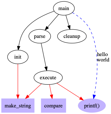
Figure 4: 设置节点和边的属性

完整的属性列表可以参考：https://graphviz.org/doc/info/attrs.html

2.2. 节点和边的布局位置（时间线实例）

默认，节点的位置是自动布局的。

通过 {rank=same; n1 n2} 可以把节点 n1，n2 固定在同一行。下面是个例子（摘自 https://stackoverflow.com/questions/61550137/using-graphviz-yed-to-produce-a-timeline-graph ）：

digraph shells {
    node [fontsize=24, shape = plaintext]; // 设置 plaintext 就没有椭圆边框了

    // 定义时间线上的节点
    1972 -> 1976;
    1976 -> 1978;
    1978 -> 1980;
    1980 -> 1982;
    1982 -> 1984;
    1984 -> 1986;
    1986 -> 1988;
    1988 -> 1990;
    1990 -> future;

    node [fontsize=20, shape = box];
    // 定义同一行的节点
    { rank=same;  1976 Mashey Bourne; }
    { rank=same;  1978 Formshell csh; }
    { rank=same;  1980 esh vsh; }
    { rank=same;  1982 ksh "System-V"; }
    { rank=same;  1984 v9sh tcsh; }
    { rank=same;  1986 "ksh-i"; }
    { rank=same;  1988 KornShell Perl rc; }
    { rank=same;  1990 tcl Bash; }
    { rank=same;  "future" POSIX "ksh-POSIX"; }

    // 连线
    Thompson -> Mashey;
    Thompson -> Bourne;
    Thompson -> csh;
    csh -> tcsh;
    Bourne -> ksh;
    Bourne -> esh;
    Bourne -> vsh;
    Bourne -> "System-V";
    Bourne -> v9sh;
    v9sh -> rc;
    Bourne -> Bash;
    "ksh-i" -> Bash;
    KornShell -> Bash;
    esh -> ksh;
    vsh -> ksh;
    Formshell -> ksh;
    csh -> ksh;
    KornShell -> POSIX;
    "System-V" -> POSIX;
    ksh -> "ksh-i";
    "ksh-i" -> KornShell;
    KornShell -> "ksh-POSIX";
    Bourne -> Formshell;

    edge [style=invis];  // invis 是“不可见”，之所以定义它们，是为了调整位置
    1984 -> v9sh -> tcsh ;
    1988 -> rc -> KornShell;
    Formshell -> csh;
    KornShell -> Perl;
}

上面代码可以生成图 5。

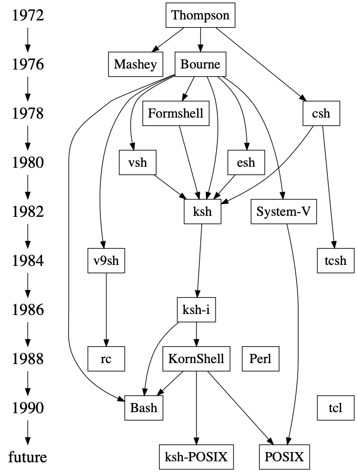
Figure 5: 时间线例子

2.3. record 形状

graphviz 支持 record 形状。

考虑 dot 文件：

digraph structs {
  node [shape=record];  // 设置默认为 record 形状

  struct1 [label="<f0> left|<f1> middle|<f2> right"];
  struct2 [label="<f0> one|<f1> two"];
  struct3 [label="hello\nworld |{ b |{c|<here> d|e}| f}| g | h"];

  // 连线
  struct1:f1 -> struct2:f0;
  struct1:f2 -> struct3:here;
}

上面代码可以生成图 6。

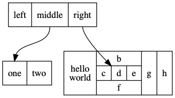
Figure 6: shape=record

2.3.1. 节点的布局走向从左到右（Hash 表实例）

默认节点的布局走向是从上到下，设置 rankdir=LR; 可以改为“从左到右”。

考虑 dot 文件：

digraph G {
  nodesep=.05;
  rankdir=LR;   // 设置布局走向从左到右
  node [shape=record,width=.1,height=.1];    // 设置默认形状为 record 等

  node0 [label = "<f0> |<f1> |<f2> |<f3> |<f4> |<f5> |<f6> | ",height=2.5];
  node [width = 1.5];                        // 设置默认宽度
  node1 [label = "{<n> n14 | 719 |<p> }"];
  node2 [label = "{<n> a1 | 805 |<p> }"];
  node3 [label = "{<n> i9 | 718 |<p> }"];
  node4 [label = "{<n> e5 | 989 |<p> }"];
  node5 [label = "{<n> t20 | 959 |<p> }"] ;
  node6 [label = "{<n> o15 | 794 |<p> }"] ;
  node7 [label = "{<n> s19 | 659 |<p> }"] ;

  // 连线
  node0:f0 -> node1:n;
  node0:f1 -> node2:n;
  node0:f2 -> node3:n;
  node0:f5 -> node4:n;
  node0:f6 -> node5:n;
  node2:p -> node6:n;
  node4:p -> node7:n;
}

上面代码可以生成图 7。

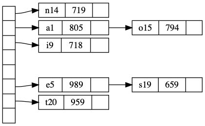
Figure 7: Hash table

2.4. UML 实例

要画 UML 图，更推荐使用 PlantUML 或者 DOTUML，这两个工具的后端都使用了 DOT，比直接使用 DOT 更方便。

2.5. 有限自动机实例

下面是有限自动机实例（摘自：https://graphviz.org/Gallery/directed/fsm.html ）：

digraph finite_state_machine {
	rankdir=LR;
	size="8,5"
	node [shape = doublecircle]; LR_0 LR_3 LR_4 LR_8;
	node [shape = circle];
	LR_0 -> LR_2 [ label = "SS(B)" ];
	LR_0 -> LR_1 [ label = "SS(S)" ];
	LR_1 -> LR_3 [ label = "S($end)" ];
	LR_2 -> LR_6 [ label = "SS(b)" ];
	LR_2 -> LR_5 [ label = "SS(a)" ];
	LR_2 -> LR_4 [ label = "S(A)" ];
	LR_5 -> LR_7 [ label = "S(b)" ];
	LR_5 -> LR_5 [ label = "S(a)" ];
	LR_6 -> LR_6 [ label = "S(b)" ];
	LR_6 -> LR_5 [ label = "S(a)" ];
	LR_7 -> LR_8 [ label = "S(b)" ];
	LR_7 -> LR_5 [ label = "S(a)" ];
	LR_8 -> LR_6 [ label = "S(b)" ];
	LR_8 -> LR_5 [ label = "S(a)" ];
}

上面代码可以生成图 8。

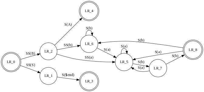
Figure 8: 有限自动机

2.6. 子图

使用 subgraph 可以定义子图。

考虑 dot 文件：

digraph G {
  subgraph cluster0 {
    node [style=filled,color=white];
    style=filled;
    color=lightgrey;
    a0 -> a1 -> a2 -> a3;
    label = "process #1";
  }
  subgraph cluster1 {
    node [style=filled];
    b0 -> b1 -> b2 -> b3;
    label = "process #2";
    color=blue
  }
  start -> a0;
  start -> b0;
  a1 -> b3;
  b2 -> a3;
  a3 -> end;
  b3 -> end;
}

上面代码可以生成图 9 。

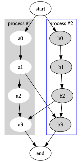
Figure 9: subgraph 实例

2.6.1. 函数调用关系实例

再考虑更复杂一点的子图：

digraph G {
size="8,6"; ratio=fill; node[fontsize=24];

ciafan->computefan; fan->increment; computefan->fan; stringdup->fatal;
main->exit; main->interp_err; main->ciafan; main->fatal; main->malloc;
main->strcpy; main->getopt; main->init_index; main->strlen; fan->fatal;
fan->ref; fan->interp_err; ciafan->def; fan->free; computefan->stdprintf;
computefan->get_sym_fields; fan->exit; fan->malloc; increment->strcmp;
computefan->malloc; fan->stdsprintf; fan->strlen; computefan->strcmp;
computefan->realloc; computefan->strlen; debug->sfprintf; debug->strcat;
stringdup->malloc; fatal->sfprintf; stringdup->strcpy; stringdup->strlen;
fatal->exit;

subgraph "cluster_error.h" { label="error.h"; interp_err; }

subgraph "cluster_sfio.h" { label="sfio.h"; sfprintf; }

subgraph "cluster_ciafan.c" { label="ciafan.c"; ciafan; computefan;
increment; }

subgraph "cluster_util.c" { label="util.c"; stringdup; fatal; debug; }

subgraph "cluster_query.h" { label="query.h"; ref; def; }

subgraph "cluster_field.h" { get_sym_fields; }

subgraph "cluster_stdio.h" { label="stdio.h"; stdprintf; stdsprintf; }

subgraph "cluster_<libc.a>" { getopt; }

subgraph "cluster_stdlib.h" { label="stdlib.h"; exit; malloc; free; realloc; }

subgraph "cluster_main.c" { main; }

subgraph "cluster_index.h" { init_index; }

subgraph "cluster_string.h" { label="string.h"; strcpy; strlen; strcmp; strcat; }
}

上面代码可以生成图 10。

Figure 10: subgraph 实例 2

3. Tips

3.1. 设置连接点的位置

我们可以设置连接点的位置，如：

digraph G {
  a -> b [headport=s, tailport=se] // 设置连接点的位置（"n", "ne", "e", "se", "s", "sw", "w" or "nw"）
  c:se -> d:s                      // 同上，另一种写法
  e -> f                           // 对比
}

上面代码可以生成图 11。

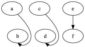
Figure 11: 设置连接点的位置

3.2. 圆角矩形（shape=Mrecord）

设置 shape=Mrecord 可以指定为形状为“圆角矩形”：

digraph mrecord {
 node [shape=Mrecord, color="skyblue", style="filled"];   // shape=Mrecord 为圆角矩形
 edge [arrowhead=vee];

 start -> running;
 start -> end;
 running -> end;

 start[label="开始"];
 end[label="结束"];
 running[label="运行"];
}

上面代码可以生成图 12。

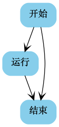
Figure 12: 圆角矩形

其它的 shape，可参考：http://www.graphviz.org/doc/info/shapes.html

Graphviz

Table of Contents

1. Graphviz 简介

1.1. DOT Language

1.2. dot 命令

2. Graphviz 实例

2.1. 节点和边的属性

2.2. 节点和边的布局位置（时间线实例）

2.3. record 形状

2.3.1. 节点的布局走向从左到右（Hash 表实例）

2.4. UML 实例

2.5. 有限自动机实例

2.6. 子图

2.6.1. 函数调用关系实例

3. Tips

3.1. 设置连接点的位置

3.2. 圆角矩形（shape=Mrecord）